RandomName2023.github.io

Response to Reviewer #23fs Q1

Q1 “Assumption 2 is too strong. Previous studies (e.g., Zhang and Sabuncu) have shown that noise robust losses usually worsen the converged solution compared to standard cross-entropy when used on clean datasets, so it’s hardly the truth that they actually lead to similar optima. I believe Assumption 2 is actually what requires more formal proofs. The empirical validation presented in D.1 is not convincing since similar training curve trends do not imply similar global/local optima.”

Thank you for your comments, we agree that more support evidence is needed for Assumption 2, and we provide them in the following. Besides, since the figures cannot be shown in the response block, which includes some important analysis(e.g. 3D visualization of the loss surface), we have attached them to Appendix C in the latest version for your reference.

1.The claim made in (Zhang and Sabuncu) is not that the robust loss functions lead to worse converged solutions, but they are actually harder to converge from the optimization point of view. We support the point from two aspects:

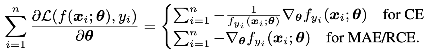
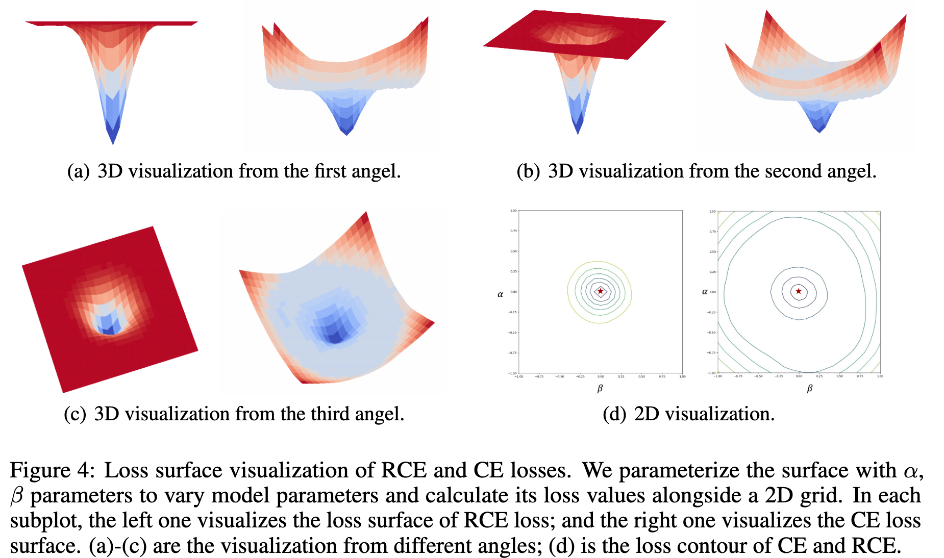
       First, the cause of difficulty in the optimization of robust loss are: (1) In the mentioned paper(Zhang and Sabuncu), they show that the gradients of the cross-entropy loss have an implicit weighting term(as shown in the following equation), which is inversely proportional to the ground-truth label’s corresponding entry at the classifier’s output. In other words, the CE loss prioritizes the harder samples during training. On the other hand, this weighting does not exist in noise robust loss functions, which means these functions treat all samples equally. The lack of implicit weighting is what (Zhang and Sabuncu) claim to be the cause of difficulty in training. (2) Our experiment in the following shows that the surface of the robust loss has a wide flat region, so when the parameters are not close to the optimal solution, the gradients could vanish, which leads to difficulty in optimization (this is verified via more extensive experiments below). For the 3D visualization of the loss surface, please refer to Appendix Figure 4 in the current version. More details about drawing the figure are shown in Appendix C.1.2.

             

      

（Left subfigure: loss curve of rce loss; Right subfigure: loss curve of ce loss. We parameterize the surface with α, β parameters to vary model parameters and calculate its loss values alongside a 2D grid.）

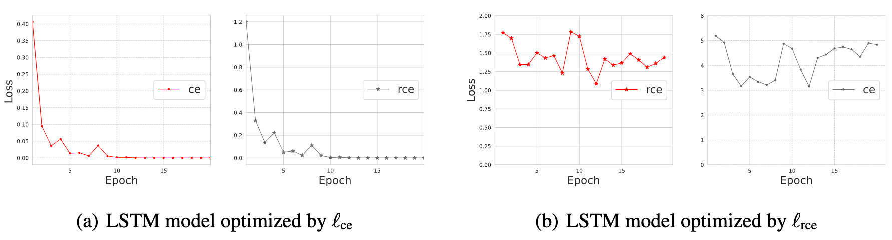
       Second, we verify the performance degradation when training the network with robust loss is caused by optimization difficulty, rather than the lack of good solution, via the following experiment: We train two networks on a standard IMDb training set: one with CE loss and another with RCE loss, and for both networks, we track the values of CE and RCE losses calculated over the training set (please refer to Appendix Figure 5). We can clearly see that when optimizing the network with CE, both CE and RCE continue to decline throughout the training, and reach the plateau at the same time, which means that the RCE loss does have a good solution. On the other hand, when training with RCE, both CE, and RCE hardly decrease, this further verifies that RCE is difficult to optimize when training the network.

      

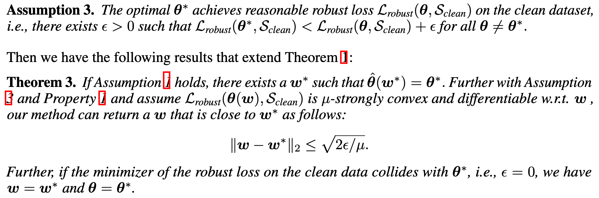
2.Theoretically, we further relax Assumption 2 to Assumption 3, which only requires the optimal solution of CE loss to also achieve a reasonably small value for RCE loss, which is within difference from the optimal value of RCE loss. Based on Assumption 3, we have extended Theorem 1 to Theorem 3 and added detailed proof in Appendix B. Assumption 3 is also supported by the following experiments.

      

3.The loss surfaces of CE and RCE losses show the two loss functions have close optimal solutions (please refer to Figure 4 in the Appendix). More specifically, we plot the loss surfaces of CE and RCE losses centered around the optimal solution of CE loss following (Li et al., 2018), which visualizes the loss surface by perturbing the network parameters along two randomly sampled directions. The procedure can be formulated as below: , where is the model parameters trained to convergence with CE loss, and are the random directions in the vector space of model parameters. α and β are the scaling coefficients of the two directions, which control how far the parameters are perturbed. We parametrize the surface w.r.t the values of α, β ranging from [-1, 1], and calculate the loss values at different positions alongside a 2D grid.

From the plot (d), we can see that the optimal solution of CE is also close to the optimal solution of RCE (also has the lowest value near zero), which is direct experimental support for Assumption 3. In addition, when the solution is not close to the optimal position, the rce loss surface is flat and wide, which is the cause of optimization difficulty.

      

We also want to note that apart from the theoretical analysis, our SunGen indeed brings considerable performance boosts over the competing methods(as shown in the main experiments). We believe our proposed framework is a good contribution to the PLM-based zero-shot learning direction. Many thanks for pointing out this issue and for the good suggestion. We have attached the above analysis and the further relaxation of Assumption 2 in the current version appendix B & C.